As the title suggests, this project saw me extend some of my linear algebra knowledge with inspiration from a course I took in 2020. Here, simple face recognition is demonstrated, a timeseries is analyzed and other interesting applications are discussed.

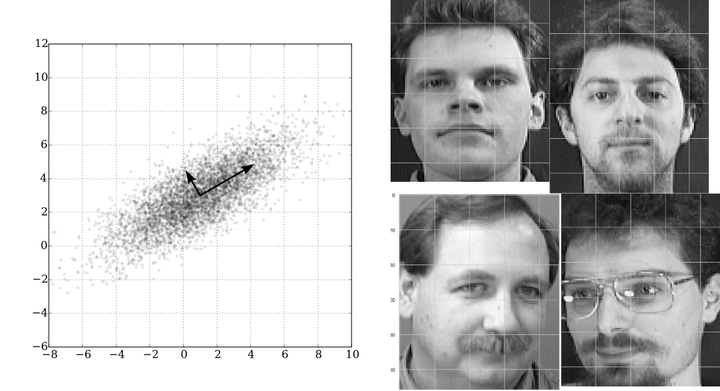
Principal Component Analysis (PCA) is a way of capturing most of the variance in the data (in an orthogonal basis). It reduces dimensions and transforms the data linearly into new properties that are not correlated. Singular Value Decomposition (SVD) will be utilized to diagonalize the matrices from which the basis vectors will be truncated to give us our principal components.

Equations

Assuming a $m \times n$ matrix $X$, the principal components are defined as the eigenvectors of the dataset’s covariance matrix. Assuming $\hat{X}$ is the dataset centered at the origin, it can be said that $\hat{X}^{T}\hat{X}$ is proportional to the covariance matrix which means finding the eigenvectors for $\hat{X}^{T}\hat{X}$ is enough. These are represented by the columns of V in the reduced SVD of $\hat{X}$,

$$\hat{X} = U\Sigma V^{T}$$

Face Recognition

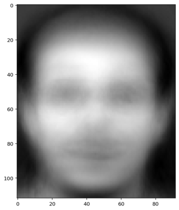
For this analysis I used, AT&T Laboratories Cambridge’s “Database of Faces”, a set of gray scale face images (like in the image above) normalized to the same resolution. Each image is a flattened row of a larger ‘faces’ matrix. First, to zero center the faces matrix, an average face is computed and subtracted from each row of the matrix. The ‘average’ face is shown below.

Using SVD, we can calculate the eigenbasis of the desired covariance matrix.

U, S, Vt = la.svd(faces_zero_centered, full_matrices=False)
V = Vt.T

As a side note, the principal components of any one of the images in the training set can be captured by converting them into the eigenface basis using the V vector found above.

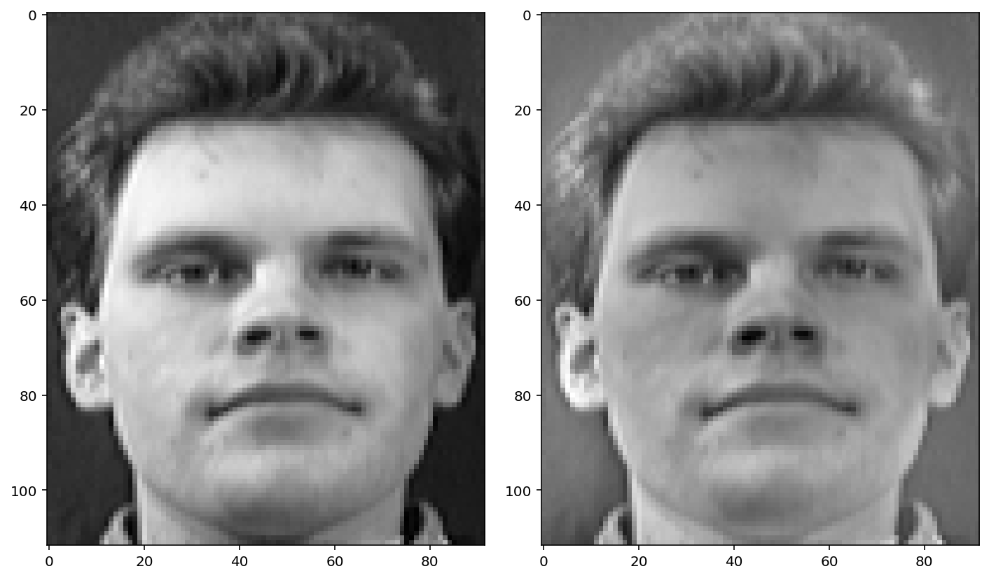
Now, with an unknown face (left) that the model is not trained on, first we will subtract the average face from it. The resulting image (right) will then be converted to the eigenface basis by a simple linear transformation.

unknown_zero_centered = face_unknown - face_avg
unknown_basis = unknown_zero_centered @ V
faces_basis = faces_zero_centered @ V

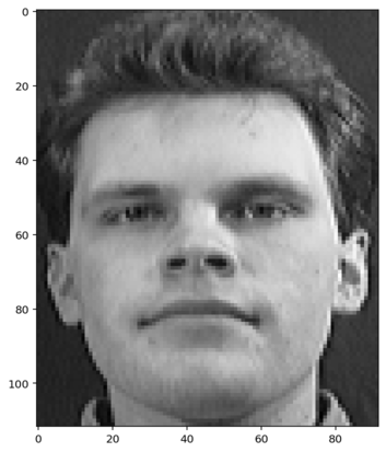
To match an existing image, the “closest” face in the face basis will be selected on the basis of least distance between the vectors.

n = 0
differences= la.norm(faces_basis - unknown_basis, axis=1)
n = np.argmin(differences)
plt.imshow(faces[n].reshape(face_shape), cmap="gray")

The above demonstration was a simple implementation of PCA on a data set of images where its assumed each face fills out a similar area in the image. Check out this link for a more complex implementation involving a trained neural net and scikit-learn

Short Example of Timeseries

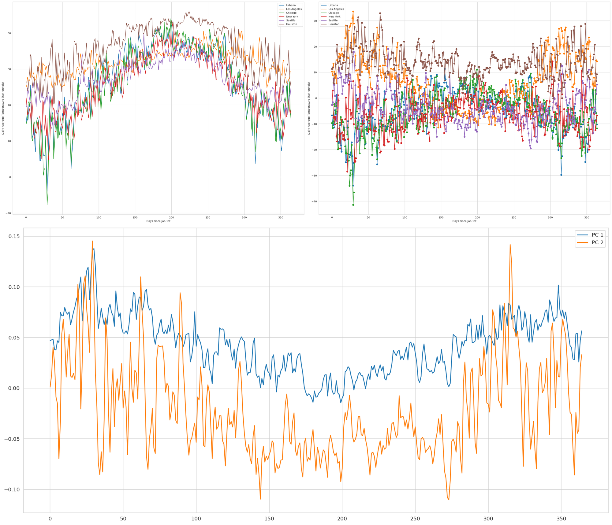
PCA can be used to split up various timeseries too. In the image below, the temperature data for six US cities is plotted (top left). Next, The average is subtracted to zero center the data like in the steps above (top right). Finally, the data is broken into its top two PCs (bottom).

# zero center the data
temp_avg = np.mean(temperature,axis=0)
temp_zero_center = temperature - temp_avg

# SVD breakdown
U,S, Vt = la.svd(temp_noavg)
V = Vt.T

# plotting the first two eigenvectors
plt.figure(figsize=(20,10))
lines = plt.plot((V[:,:2] ), '-', )
plt.legend(iter(lines), map(lambda x: f"PC {x}", range(1,6)))

Since average temperature dips in the winter and peaks in the summer, the first component represents climates that remains relatively static year-round.

Further Reading:

1. Markov Matrics was one of the coolest take aways in linalg. This article breaks down the concept and its applications in data science.
2. Briefly mentioned in the above article, Google PageRank utilizes a special kind of square matrix called the Google Matrix
3. Sandeep Khurana explains Linear Regression quite eloquently here.